Attention is all you need

Introduction

This blog attemps to provide the simple overview about the operation that happens inside Vanilla Transformers as mentioned in “Attention is all you need” paper. i.e. computations inside the transformer. PyTorch implementation of the paper can be found here.

This paper introduced the concept of Transformer model architecture, which has become a foundational model in NLP tasks. The most fundamental concept in transformer architecture is the_ self-attention _mechanism. On surface level, self-attention is just another sequence-to-sequence operation i.e. It takes sequence as input and return sequence as output. But it is really powerful because of its ability to perform parallel computation and preserve long-term dependencies.

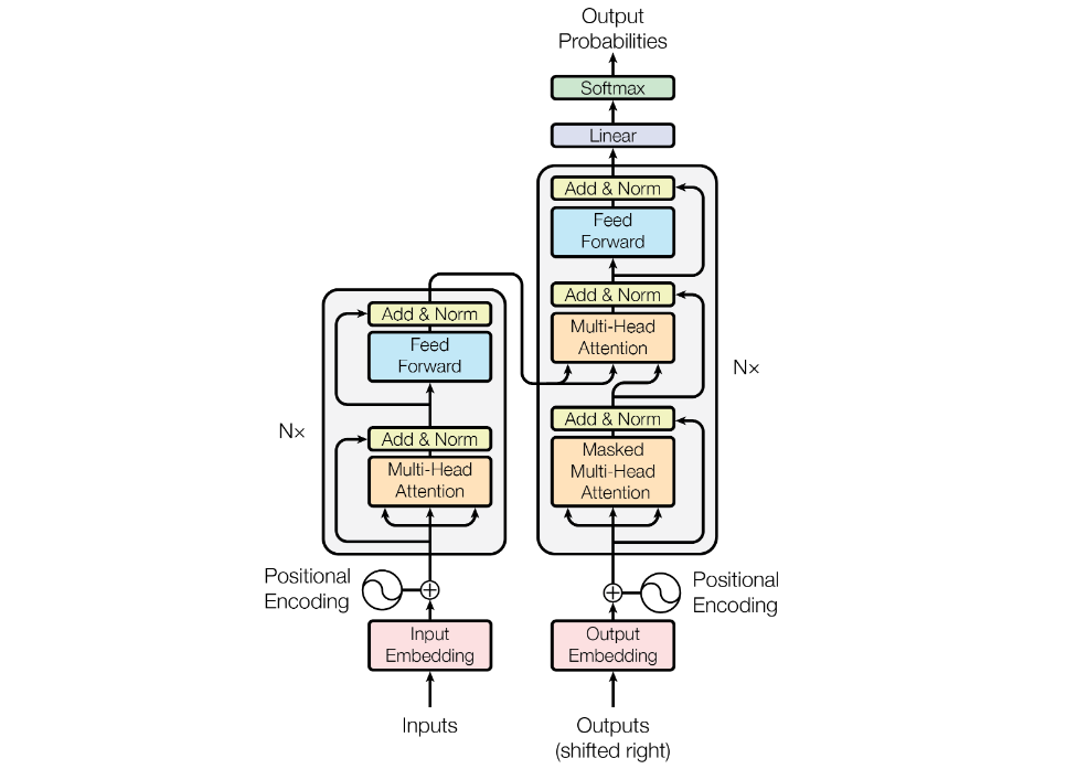
The above image shows transformer architecture with encoder and decoder. The original paper was introduced for neural machine translation task.

Now, Let’s try to understand the Transformer.

Word Encoding/Representation

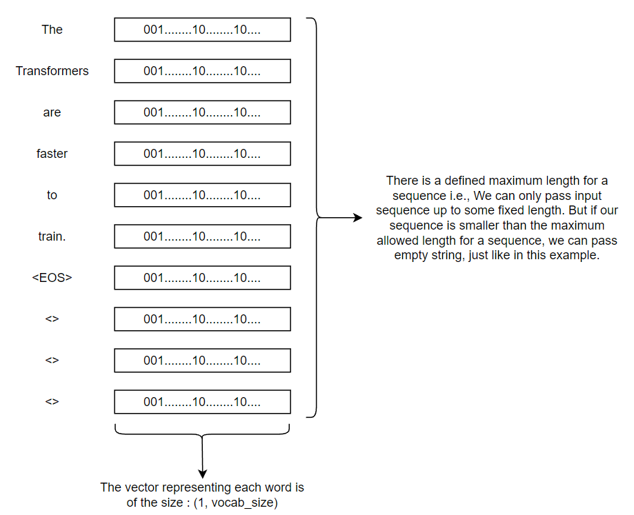
At first, each input word is represented/encoded into some vectors. All the encoded vectors are of the same shape. And since the transformer model takes a fixed length sequence as input, the smaller length sequence is increased to that fixed length by padding empty strings just like in the diagram below.

Word Embedding

Computers are unable to understand words. So, we need to represent the words as dense, low–dimensional vectors in a continuous vector space. The main idea of word embeddings is to capture the semantic and syntactic relationship between words. The embeddings are learned from large amounts of text data using unsupervised machine learning techniques. For Example : We take a paragraph, mask some portion of that paragraph, force the model to predict the masked part and repeat it multiple times. As a side effect of this, we are able to capture meaning and relationship between words by representing the word as an embedding vector.

Input Embedding

Now, we pass our word representations to the word embeddings in a feed forward layer and obtain the embeddings for our input. The dimension of embeddings is described to be 512 in the original paper.

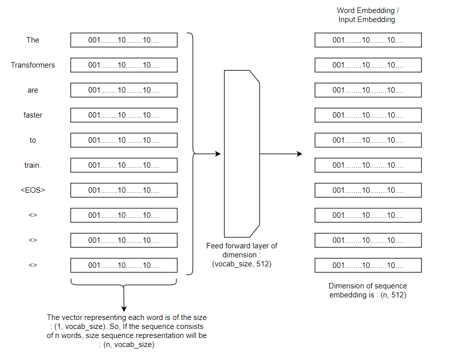
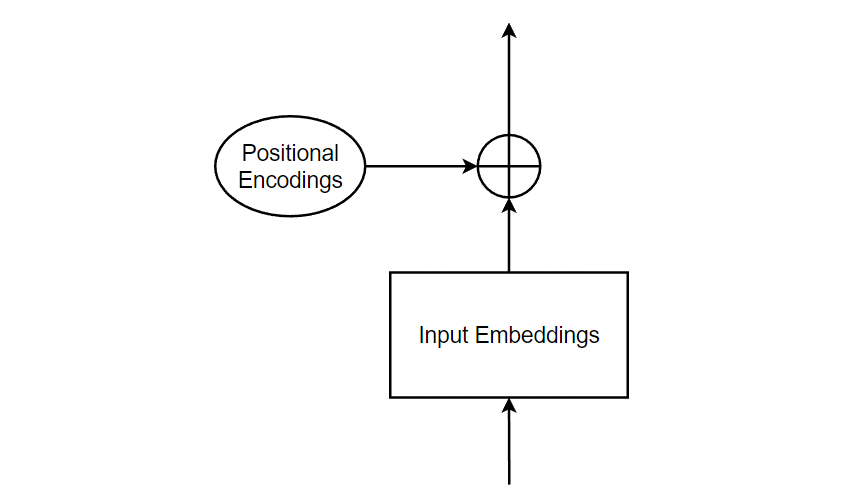
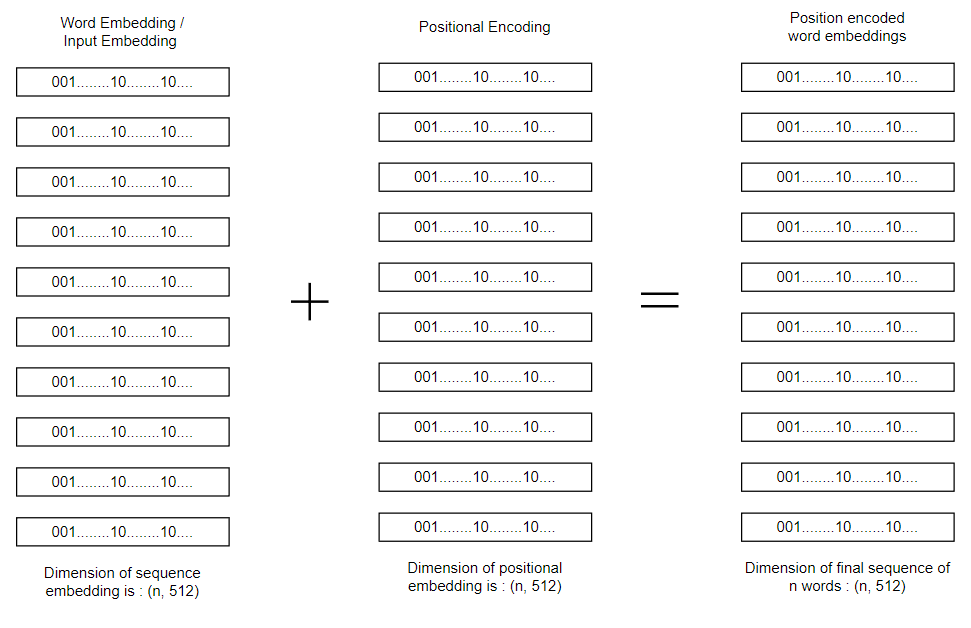
Now, we have generated input embeddings. Next step is to add the input embeddings with positional encodings.

Positional Encodings

Since we’re dealing with natural language, the positions and order of the words are extremely important as sentences follow grammatical rules and different order of the same words can give different meanings. In transformer models, each word in a sentence flows through the encoder/decoder stack simultaneously and the model itself doesn’t have any sense of position/order for each word. Therefore, there’s a need to incorporate the order of the words into the model.

But in the vanilla Transformers, we use positional encodings.

Even if both the positional embeddings and positional encodings are for the same purpose, we need to understand that positional encodings are derived using some equations while positional embeddings are learned.

Positional embeddings are used as a query for masked prediction, while positional encodings are added before the first MHSA block model.

Equations to derive positional encodings for vanilla transformers are:

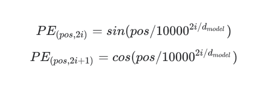
After we’ve calculated the positional encoding, it’s time to add it with the input embeddings to preserve the position of words.

Now, we’ve processed the input sequence and the next step is to pass he input to encoder. But at first, Let’s try to understand what encoder block really is?

Encoder Block

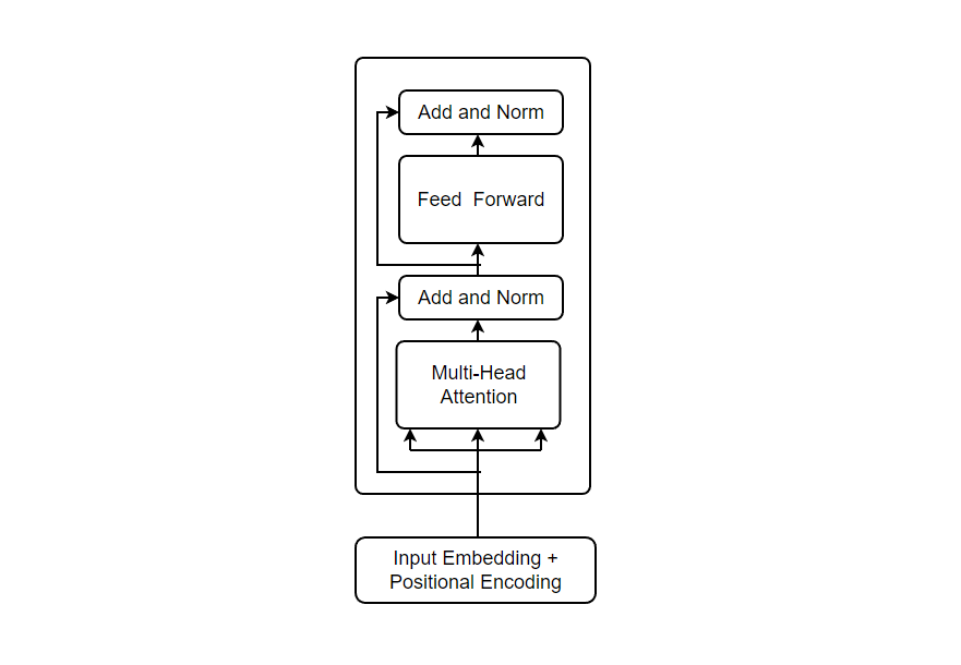
Firstly, we see our input is passed with 3 arrows to the Multi-Head Attention Block. The Multi-Head in the block means the parallel computation i.e. Inputs are processed and computation occurs parallely which increases the speed. Another reason for using Multi-Head attention is to allow the network to model all the different relations in single attention operation, and multi-head basically means attention operation applied in parallel.

But what is attention?
Attention operation is a method that includes the computation where each word is assigned attention score that tells the model about what to focus and what not to focus in order to understand the meaning of sequence. In the vanilla transformers, we use self-attention mechanism. So, Let’s learn more about it.

Self-Attention

Let’s assume a sequence “In Bayesian Inference, We update the prior probability of model using the new data.” We can easily understand the sentence because we know the meanings and the rules of grammar. But computers have absolutely no idea about what is this and what it means. The self attention mechanism will process each word, observes all the position of tokens in the sequence and create a vector trying to make sense of the sequence. Basically, it generates a vector based on dependency of words and understanding the context.

The self-attention operation starts with the inputs. Each input is representation of a single word in a sequence. For each input, we generate three different representations known as key, query & value. In order to generate these three entities, we multiply our input with some radomly initialized matrix weights for all of them. Randomly initialized weights are different for all key, query & value.

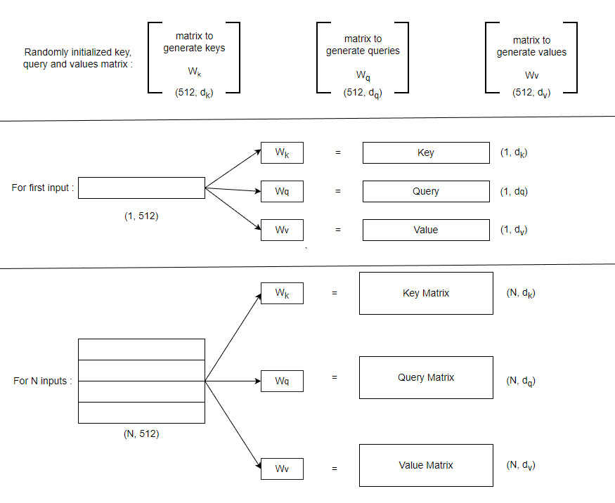
In self-attention mechanism, The dimension of key and query matrix are same i.e. 64 (mentioned in the paper) For attention operation, query and key are multiplied to obtain a single number which is again multiplied with value vector. The figure below shows how attention operation is performed.

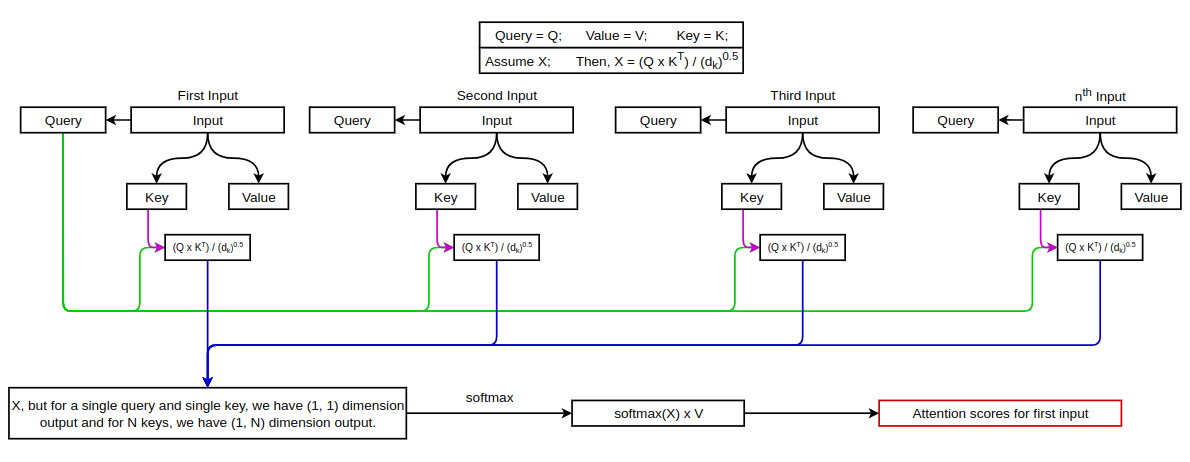
The figure above shows the attention score for first input. Now, Let’s see how it is done for second input.

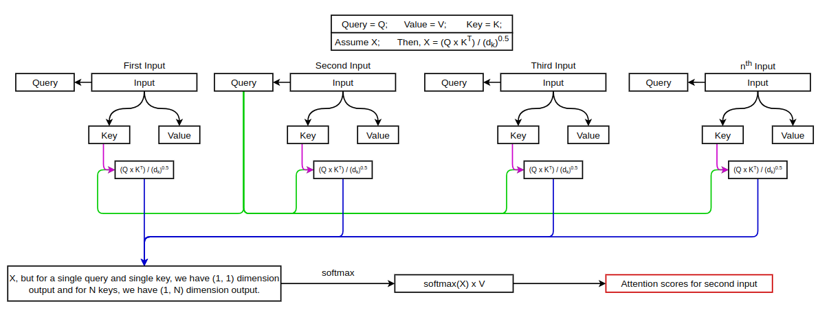
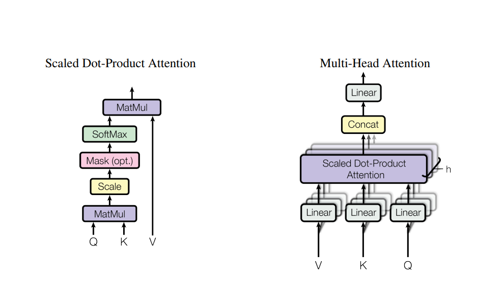
This is similar for rest of the inputs. This is the way self-attention is calculated. The attention operation we performed is called Scaled Dot-Product Attention. But, in the paper, Multi-Head Attention is used. We can see this figure from the original paper to understand the difference betwene the two.

Residual Connection and Layer Normalization

After the attention operation, residual connection is added (i.e. Input to the Mult-Head Attention block and it’s output are added.) and then we perform layer normalization.

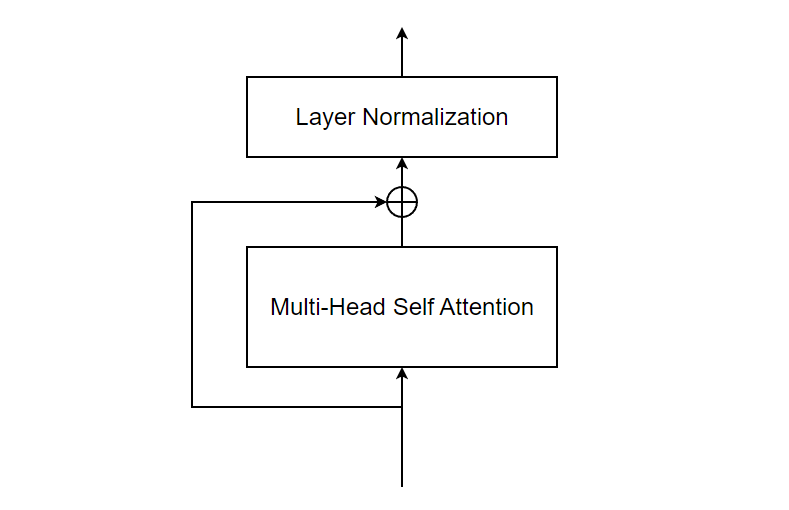
The purpose of the residual connection in the multi-head self-attention mechanism of a Transformer is to facilitate gradient flow during training and improve the overall learning capability of the model. In the context of multi-head self-attention, the residual connection is applied to the output of the self-attention module before it is passed through subsequent layers, such as feed-forward neural networks or additional self-attention layers. The residual connection allows the model to retain the original information from the input and combine it with the learned representation from the self-attention module. And the purpose of this normalization step is to ensure that the inputs to subsequent layers are consistent and within a similar range, which can help improve the overall performance and convergence of the model.

Feed Forward and Normalization

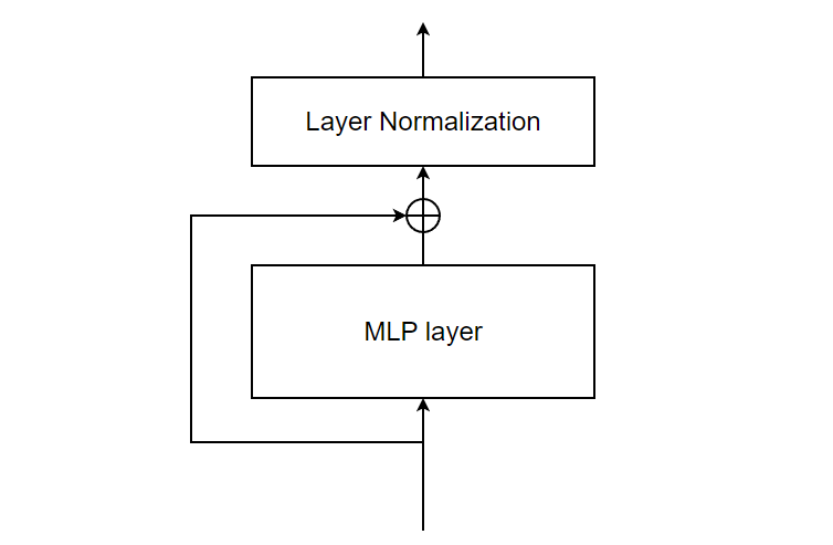
Now, the normalized output is passed through a feed forward layer (Multi-Layer perceptron) with another residual connection followed by layer normalization.

We have completed the encoder block. So, let’s move on to decoder block. Decoder block is quiet similar to Encoder except it has one extra layer called Masked Multi-Head Attention. But rest of decoder is exactly the same.

Decoder Block

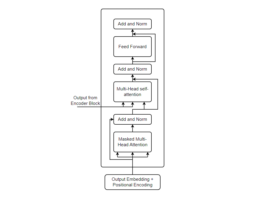
In the block diagram of decoder block above, we can see everything is same as Encoder except masked Multi-Head Self-Attention. Let’s understand it all.

Similar to the encoder block, decoder block starts with Output Embedding and Positional Encodings. The process of generating output embedding and positional encoding is exactly same as generating input embedding and positional encoding for the Encoder Block. After generating, output embedding and positional encodings, we add them together and pass the result to masked multi-head self-attention. Before passing, we generate three different representations i.e. key, query & value. The process of generating these vectors is to multiply the input to the masked MHSA block by some randomly initialized matrix weights for all of them. We studied Multi-Head Self-Attention mechanism, But, what is Masked Multi-Head Self-Attention, why is masking done??

Basically, masking is done to achieve parallelism while training. It is used to prevent the attention mechanism from looking at future tokens during the encoding process. For instance, when predicting the third word in a sentence, we should not allow the model to see the fourth or subsequent words, as that would violate the sequential nature of language. Therefore, the model masks out (ignores) the future positions during the attention calculation.

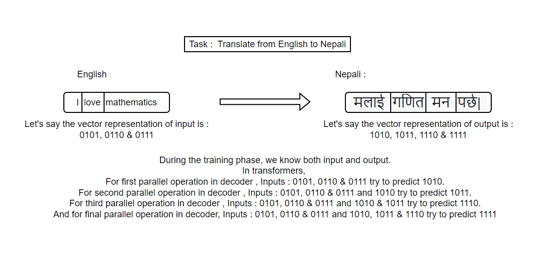
This is where masking becomes necessary. The training algorithm knows the entire expected output but it hides/masks some portion of output.

After the masked multi-head self-attention, we make residual connections and perform layer normalization. The output of this layer is used as value for next MHSA block. The output from the encoder block is used to generate two representations key & query. Now, we have all key, query and value for the MHSA block. So, we perform self-attention operation again followed by residual connection and layer normalization.

The output is further passed to a feed forward layer again followed by residual connection and layer normalization. These are all the operation inside decoder block.

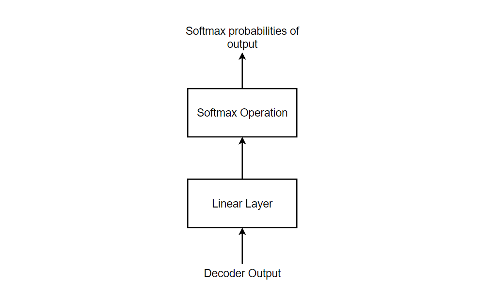
The output from decoder block is further passed to a linear layer and softmax layer and the word with highest probability is selected.

    1. The Illustrated Transformer.
    2. Illustrated Guide to Transformers- Step by Step Explanation.
    3. Transformer from scratch using pytorch.
    4. Masking in Transformers’ self-attention mechanism.
    5. Attention Is All You Need.
    6. Transformers from scratch.
    7. Illustrated: Self-Attention.
    8. Transformers from Scratch in PyTorch.
    9. Explained: Multi-head Attention (Part 1).
    10. Explained: Multi-head Attention (Part 2).
    11. Transformers Explained Visually (Part 1): Overview of Functionality.
    12. Transformers Explained Visually (Part 2): How it works, step-by-step.
    13. Transformers Explained Visually (Part 3): Multi-head Attention, deep dive.
    14. Understanding Attention Mechanism in Transformer Neural Networks.
    15. Transformer Architecture: The Positional Encoding.
    16. Word Embeddings - EXPLAINED!.
    17. A Gentle Introduction to Positional Encoding in Transformer Models.