
Bayesian Statistics - Introduction
Introduction
Before diving into the bayesian concept, let’s first understand what does it mean when something has some probability of occurring??
We can understand it in two different manner : Frequentist & Bayesian.
For example: When considering the probability of rolling a four on a fair six-sided die, we can think of it in an objective manner. If we were to roll the die an infinite number of times, take random samples, and calculate the proportion of fours observed, it would tend towards one-sixth. This means that, in the long run, the proportion of the outcome we’re interested in converges to one-sixth. So, one way to explain what is the probability of an outcome in terms of frequencies is if the event were to happen infinitely many times, what would be the proportion of outcome we’re interested in. This is simple, straightforward and sounds correct because frequentist approach reflects objective reality.
Another point to consider is the subjective approach, in which people have their own reasons for believing in a particular probability. This subjective viewpoint, which differs from the seemingly more accurate but rigidly objective viewpoint, serves as the foundation for our Bayesian model. It is not subjective in the sense of arbitrary beliefs; rather, it recognizes that various people may respond differently to the same inquiry based on experiences.
While the frequentist approach works well when picturing an endless number of dice rolls, it becomes difficult to apply it to unique one-time occurrences such as F1 Race because racing does not have a finite number of outcomes. For example, calculating the likelihood of Hamilton winning the F1 at Losail circuit requires insights that the frequentist model may not readily supply. Using a frequentist model would require imagining an infinite sequence of races, each with a different outcome, sample it and calculate the proportion of desired outcome and all of that without any background knowledge. Now, we are starting to see the flaws of the frequentist approach.
Let’s look at an example on how the bayesian approach can be subjective and true:
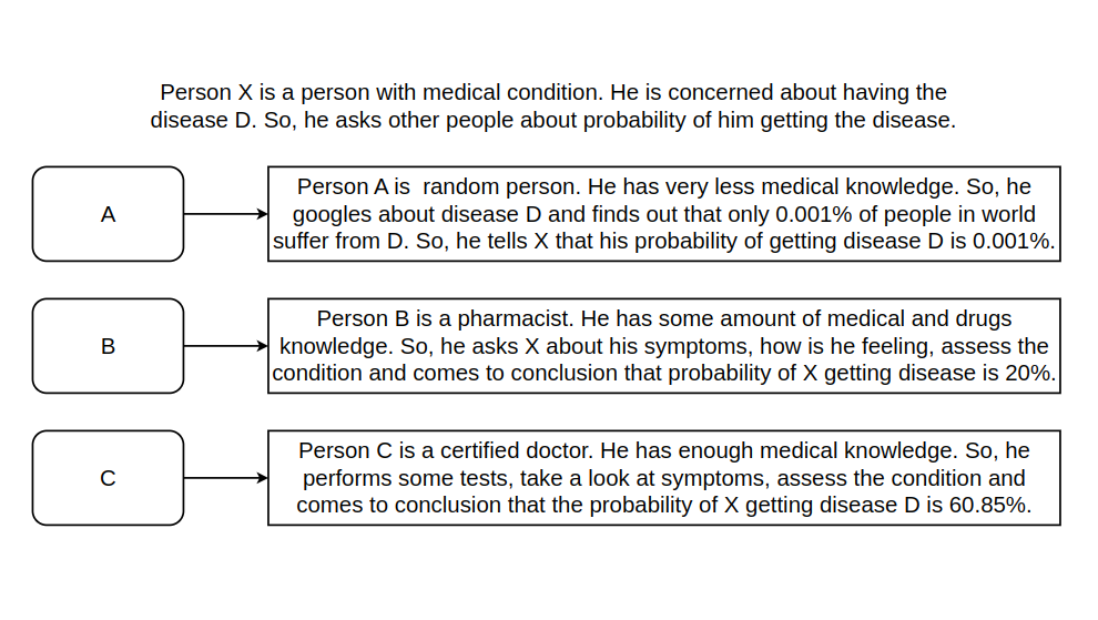
In the example above, all persons A, B & C are correct about the disease. It’s just they predicted based on the knowledge and the prior information available to them. But, A cannot say that the probability is 90% with just the information he has. The probability only gets updated after we add more and more information. The degree of belief helps form the probabilistic base of everything.
Conditional Probability
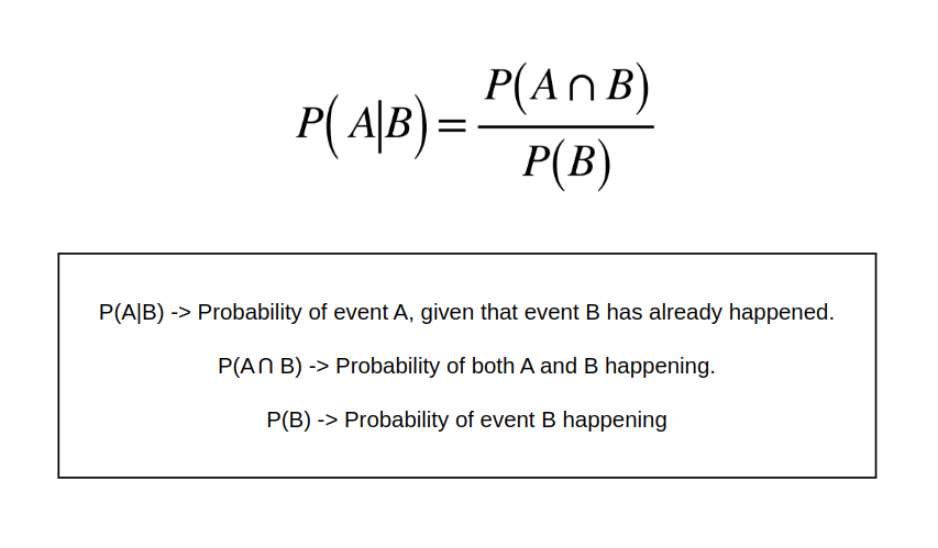
In order to get complete intuition behind the bayesian statistics, we need to understand conditional probability. Let’s say that event A and event B are related to each other. Conditional Probability is the probability of a certain outcome from event B, given that event A has already happened. Conditional probability can be expressed mathematically in following way:
For Example: Consider a class of 50 students where 15 are females, 20 are Mathematics majors and there are 8 females in Mathematics class. So,
Total Students n(T) = 50
Number of female students n(F) = 15
Number of students who are not female n(~F) = 50 - 15 = 35
Number of students who took mathematics major n(Mat) = 20
Number of students who do not took Mathematics major n(~Mat) = 50 - 20 = 30
Mathematics major who are female n(F and Mat) = 8
Mathematics major who are not female n(~F and Mat) = 20 - 8 = 12
Females who are not mathematics major n(F and ~Mat) = 15 - 8 = 7
Students who are neither female nor mathematics major n(~F and ~Mat) = 30 - 7 = 23
Let’s try to understand it using table:
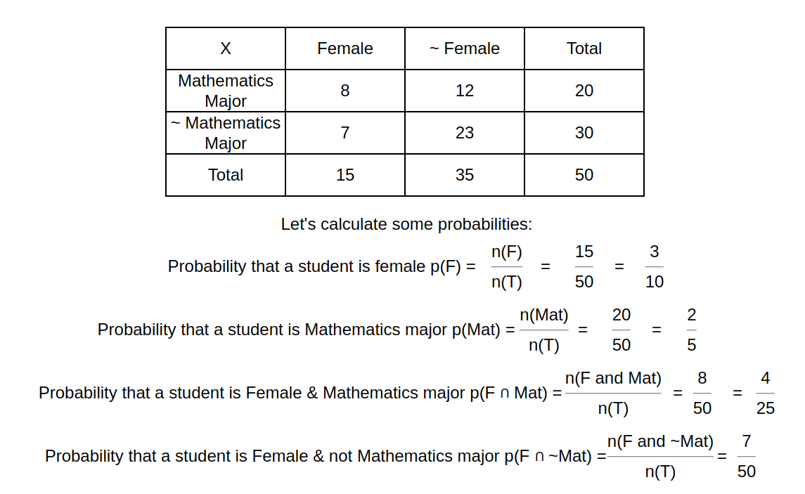
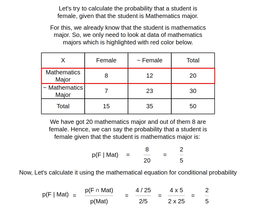
Now, let’s calculate some conditional probability using above data:

Let’s take a look at another example involving conditional probability:
Hazard loves to play football, but especially when the weather is good. The probability that he plays football is 70% when it is sunny. But when it’s raining, the probability that he plays is just 40%. He stays in London and there is a 60% chance that it is sunny on any given day. Hazard played football last wednesday. Now, what is the probability that it was sunny last wednesday?
We can try to understand it using tree diagram:
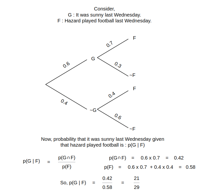
From this example we can see that normally in London, the probability of a sunny day is 60%, but given the information that Hazard played football that day, we can conclude the probability of that day being sunny is 72.41%.
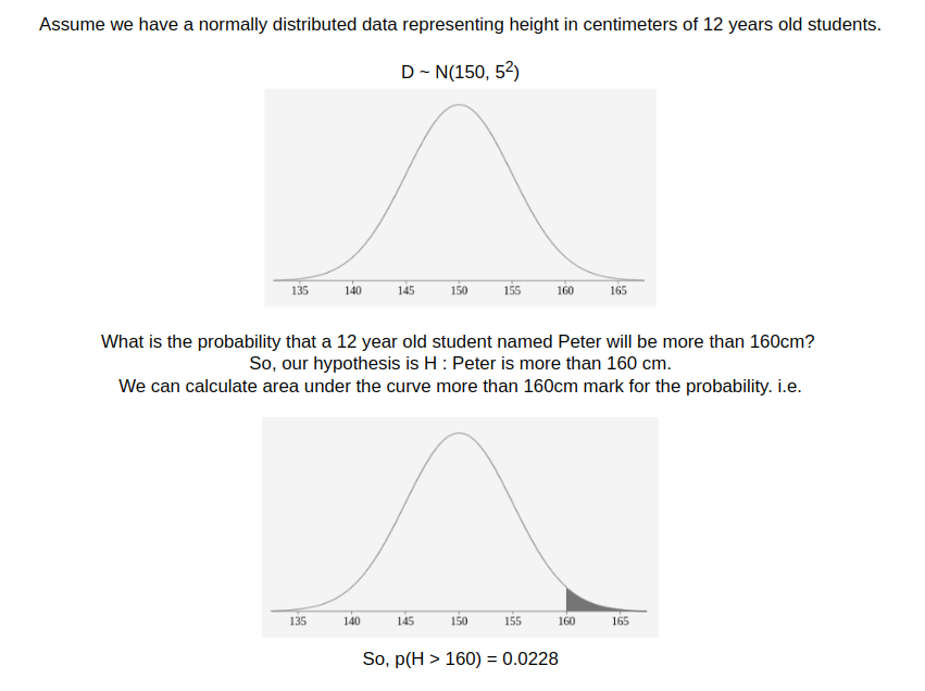
Above example involves discrete data, but in the next examples, let’s talk about conditional probability with respect to continuous examples:
Example 1:
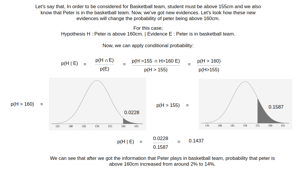
Example 2:
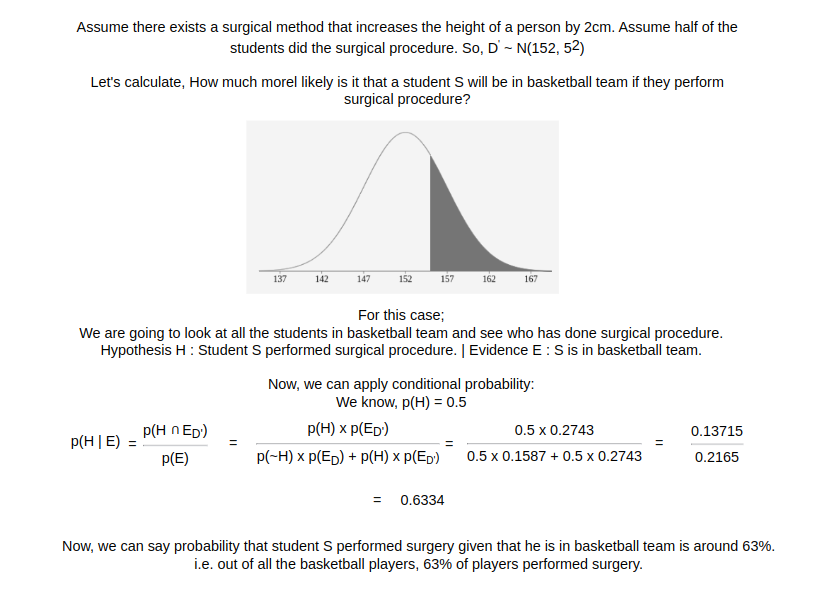
Bayes Theorem
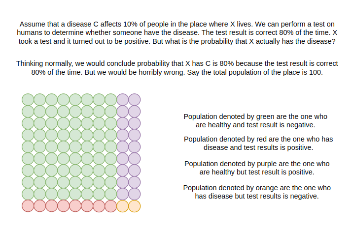
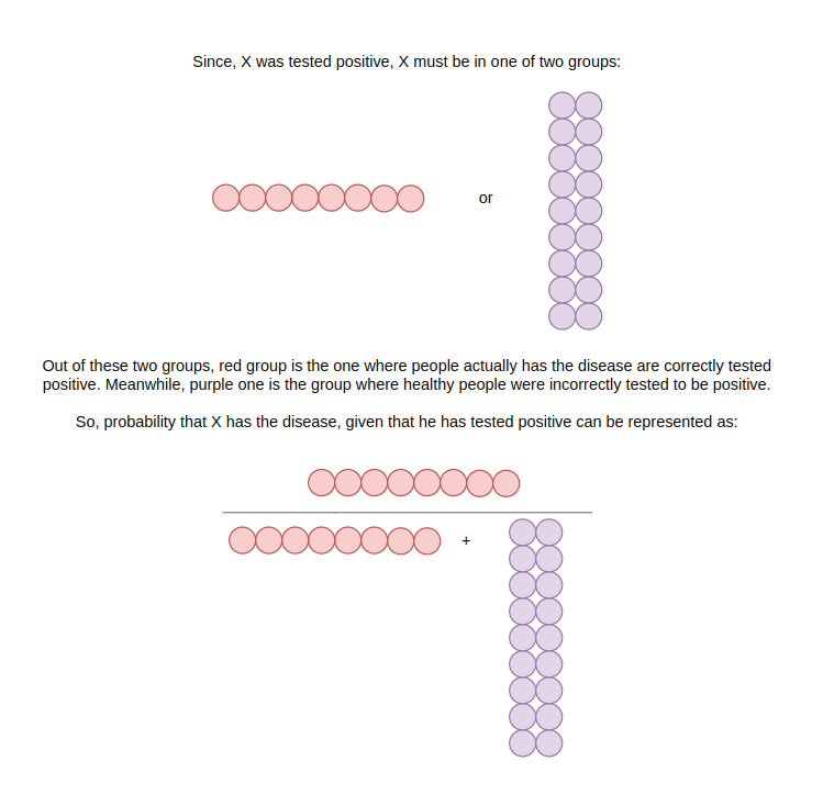
Let’s look at another example which is in fact one of the most famous examples for understanding bayes theorem.
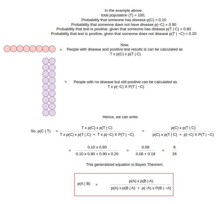
Let’s try to generalize what we did by making equations.
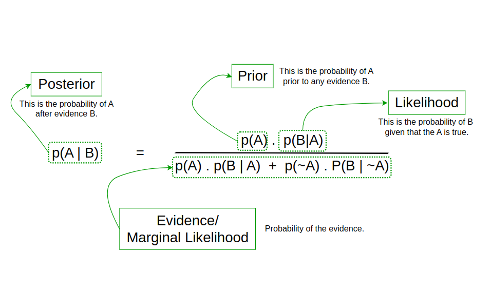
Below are the terminologies used for different parts of bayes themorem.
References for this blog (Click on references for more info):
1. Introduction to Bayesian Statistics - A Beginner’s Guide (Best resource ever).
2. Bayes theorem, the geometry of changing beliefs.
3. The medical test paradox, and redesigning Bayes’ rule.
4. A Gentle Introduction to Bayes Theorem for Machine Learning.
5. Bayes’s Theorem.
6. Conditional Probabilities, Clearly Explained!!!.
7. Bayes’ Theorem, Clearly Explained!!!!.
8. The Bayesian Trap.
9. The quick proof of Bayes’ theorem.