
Vision Transformers
Introduction
Convolutional Neural Networks (CNNs) belong to the category of deep learning models that have significantly influenced the domain of computer vision. They excel in tasks related to image analysis, recognition, and comprehension, demonstrating a strong suitability for such endeavors whereas transformer architectures are basically the architecture that uses attention mechanism at its core. Since its introduction in 2017, transformers and its variations were used for tackling the sequence problems specifically related to Natural Language Understanding & Processing including machine translation, text generation, language modeling and more. But Google Research released a paper named “An Image is worth 16 x 16 words: Transformers for Image recognition at scale” and introduced Vision Transformers (ViT), a new way of computer vision.
In this blog, we will discuss vanilla Vision Transformers. Transformers have a huge impact on the NLP domain as we can pre-train them on large corpus and then fine-tune for specific purposes without compromising efficiency, scalability & saturation in performance. Vision Transformers were primarily developed for image classification tasks. However, before ViT, transformers have not been used effectively for computer vision purposes. Before learning about vision transformers, we need to have a good understanding of Transformer architecture. For that you can check my previous blog here. PyTorch implementation of Vision Transformers can be found here. Below is the ViT architecture from the original paper.
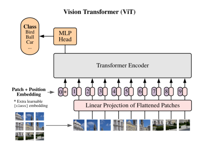
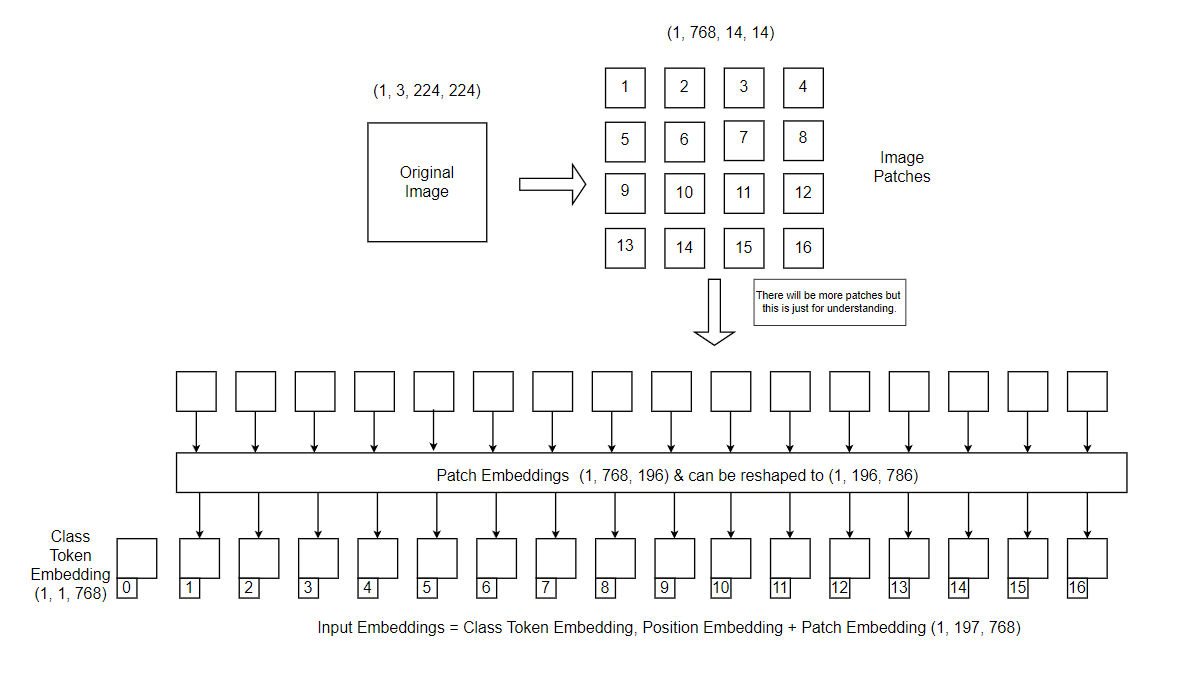
In ViT, power of the transformer is utilized in a quite different manner than CNN’s. First, the image is split into patches, flattened and positional embeddings are added. Finally, the image representation is passed through the transformer followed by classification head. Let’s try to understand it step by step.
Split image into patches
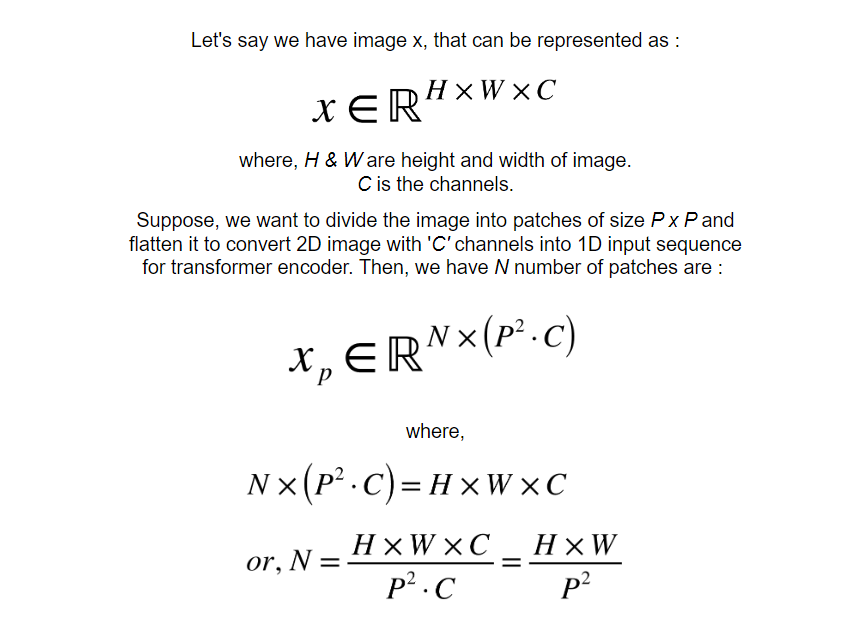
Image patches are small, rectangular subregions or segments that are extracted from a larger image. These patches represent localized portions of the image and can be thought of as smaller “pieces” of the overall image. They can be used for multiple purposes such as feature extraction, parallel processing, data augmentation & capturing spatial context.

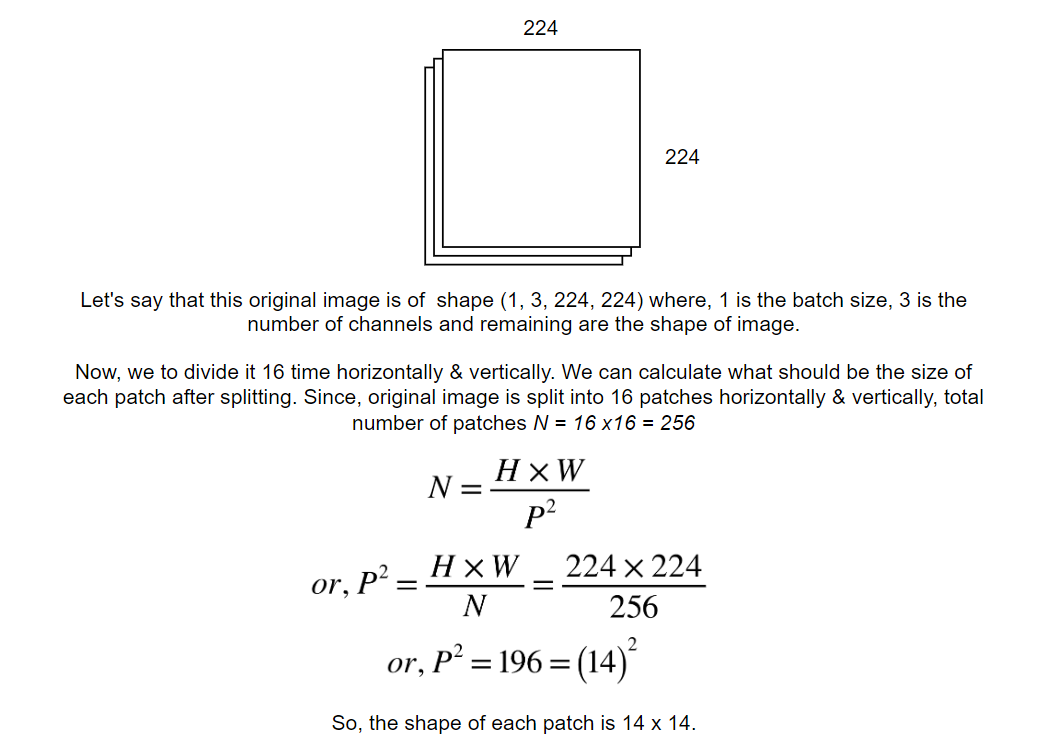
Splitting images into patches in vision transformers enables efficient processing, effective capture of both local and global context, adaptation of transformer concepts from text to images, and the ability to handle varying input sizes. This approach forms the basis for applying transformers to image data successfully. This process is done for all the channels & is performed in the following manner.
Patch Embeddings
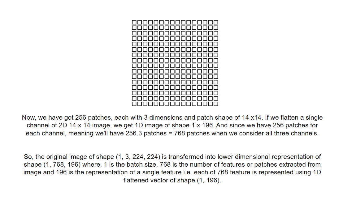
The Transformer uses constant latent vector size D through all of its layers, so we flatten the patches and map to D dimensions with a trainable linear projection i.e. it represents each image patch of size (P x P) with channel C in 1D using D latent vector size. This representation is known as patch embeddings.
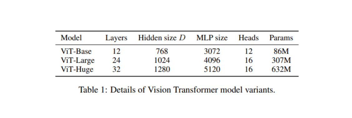
The latent vector D in our image is 768. We can learn more about different latent vector sizes in the different variations of vision transformers from the table1 of the paper which is shown below.
Position Embeddings & Extra Class Embeddings
Unlike CNNs, ViT processes images as sequences of flattened patches. However, images have a spatial structure and this information needs to be incorporated in with the input for the model to understand the relationship between different patches. So, position embeddings are introduced to address this issue. This is important because without position embeddings, the model would treat the patches as an unordered set and lose the spatial information. Furthermore, we prepend a learnable embedding, often referred as “class token” which is important for training and inference purposes. After all of these computations, we are ready to pass input embeddings to the transformer encoder.
Position embeddings are added to the patch embeddings to retain positional information. Standard learnable 1D position embeddings are used because we have not observed significant performance gains from using more advanced 2D-aware position embeddings.
During the training phase, the class token plays an important role in helping the model understand the overall content of the image and its relationship to specific patches. While computing self-attention, each patch is associated with the class token & acts as a way for the model to take into account high-level features that might be important for the final classification.
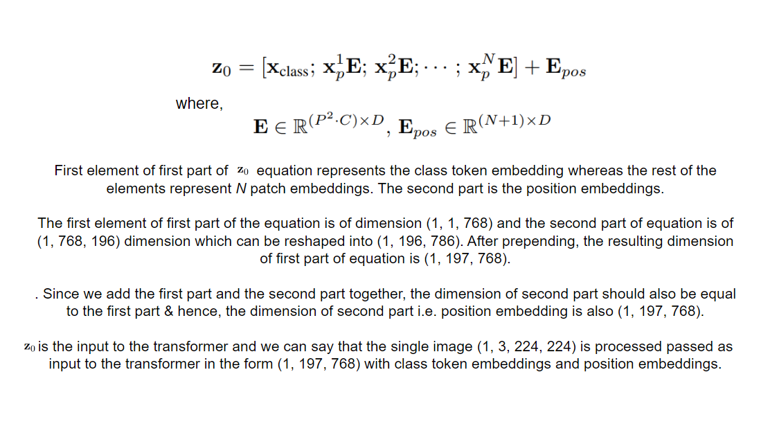
This can be represented in terms of equation:
Transformer Encoder
The transformer encoder used in ViT is a slight variation of vanilla transformers’ encoder. Let’s have a look at the difference between the two encoders.
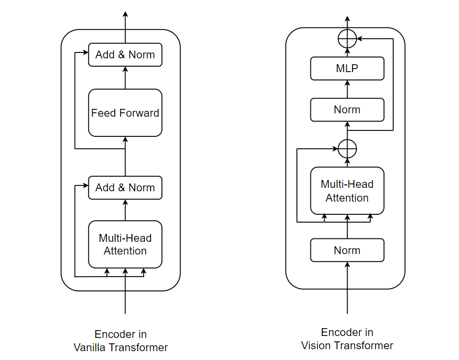
Vision Transformer Encoder block consists of four layers which consists of Multi-Headed Attention, Multi-Layer perceptron & two LayerNorm.
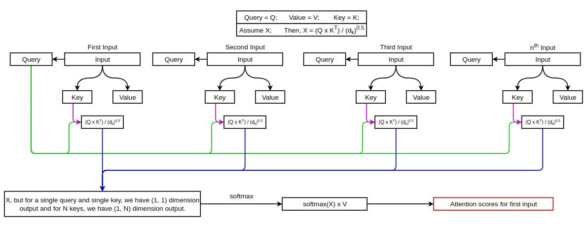
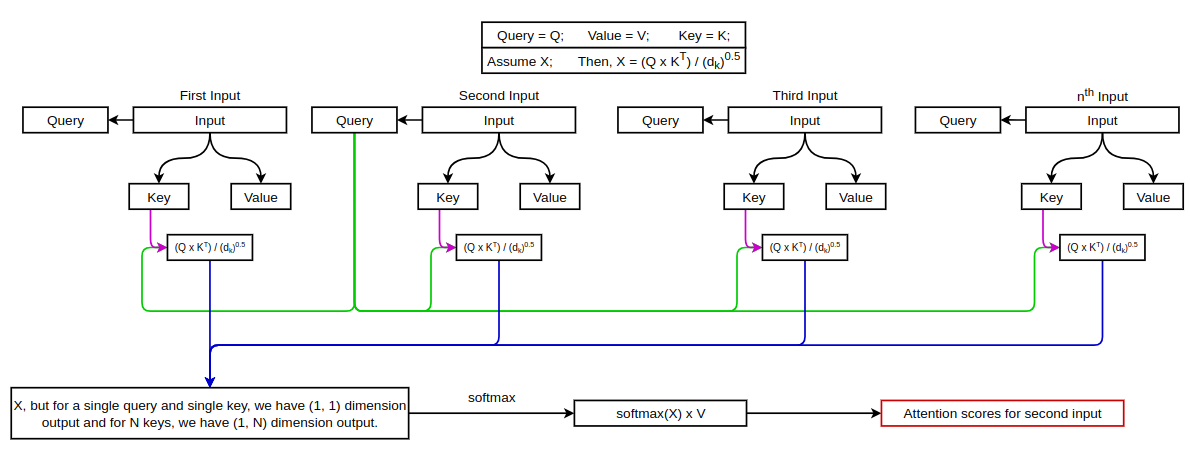
In ViT, the input embeddings are passed to the encoder layer and are normalized first. Now, similar to vanilla transformers, we randomly initialize Key, Query & Value matrices and multiply them with the normalized learnable input embeddings in order to get Key, Query and Value for our input. The process of calculating attention weights is the same as that of vanilla transformers. We can calculate the attention for each input as shown in the figure below:
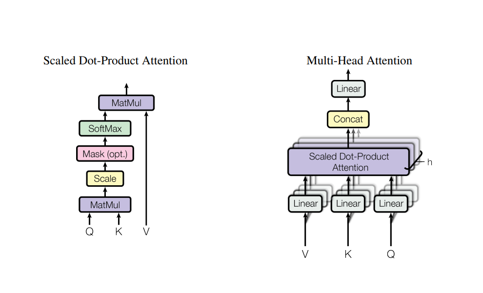
This way of calculating Attention is known as Scaled dot product attention but in the vision transformers Multi-Head Attention is used which basically means performing attention operation in parallel. We can see this figure from the original paper to understand the difference between the two.
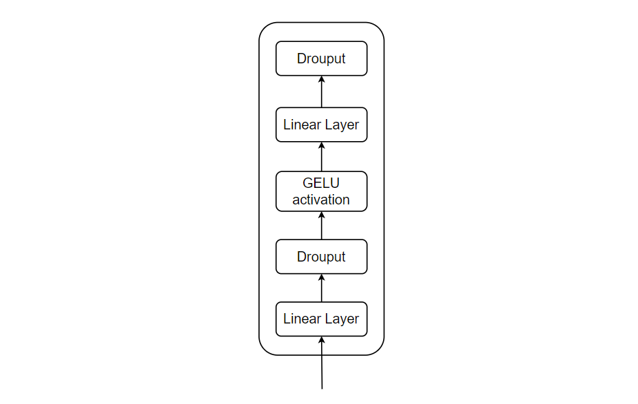
After the attention is calculated successfully, we add the attention with input embeddings that was passed to the encoder block as there is residual connection(skip connection) from the beginning of the encoder block. After this, the output is again normalized followed by a Multi-Layer perceptron (MLP) block and residual connection as shown in the block diagram of ViT Encoder. The MLP block is generally a collection of feed-forward layers. In ViT, MLP consists of two linear layers with GELU (Gaussian Error Linear Unit) non-linearity in between them and a Dropout layer after each of the linear layers.
The output from the MLP block is passed through the MLP head or sometimes referred as Classification Head. As we have added a class token on the input and it takes on representing the image at its core. The output of this token is transformed into class prediction with the help of MLP head. MLP head consists of a single hidden layer followed by a tanh activation function during pre-training and consists of a single linear layer followed by tanh activation during fine-tuning.
MLP head in ViTs produces an output distribution. In the context of ViTs, the MLP head’s final layer usually consists of units equal to the number of classes in the classification task. Each unit corresponds to a class, and the values produced by these units can be thought of as representing the model’s confidence or likelihood that the input image belongs to a particular class.
To convert these raw scores or logits into a probability distribution, a softmax activation function is often applied. The softmax function normalizes the scores across all the units (classes) and converts them into probabilities. Each probability reflects the model’s estimated probability that the input image belongs to the corresponding class. This output distribution can then be used for making predictions or for calculating the loss during training.
References for this blog (Click on references for more info):
1. AN IMAGE IS WORTH 16X16 WORDS:
TRANSFORMERS FOR IMAGE RECOGNITION AT SCALE.
2. Vision Transformers [ViT]: A very basic introduction.
3. learnpytorch.io (One of the best).
4. How the Vision Transformer (ViT) works in 10 minutes: an image is worth 16x16 words.
5. The Vision Transformer Model.
6. Vision Transformer: What It Is & How It Works.
7. Review: Vision Transformer (ViT).
8. Vision Transformers (ViT) Explained + Fine-tuning in Python.